The Petabyte Alert Stream & Observational Spectroscopy Bottleneck
In contemporary observational astrophysics, wide-field synoptic sky surveys generate streaming alert packets at rates that completely outstrip human review. The Vera C. Rubin Observatory’s Legacy Survey of Space and Time (LSST) will capture roughly 15 terabytes of optical imaging data every night, issuing upwards of 10 million transient alert packets per 24-hour cycle.
Securing follow-up spectroscopic confirmation for this astronomical torrent is physically impossible: the global fleet of 8-meter to 10-meter optical telescopes can secure spectra for less than 0.01% of detected targets. Astronomical brokers (such as ALeRCE, Fink, and ANTARES) must categorize celestial objects in real time using only broadband optical magnitudes and derived color indices.
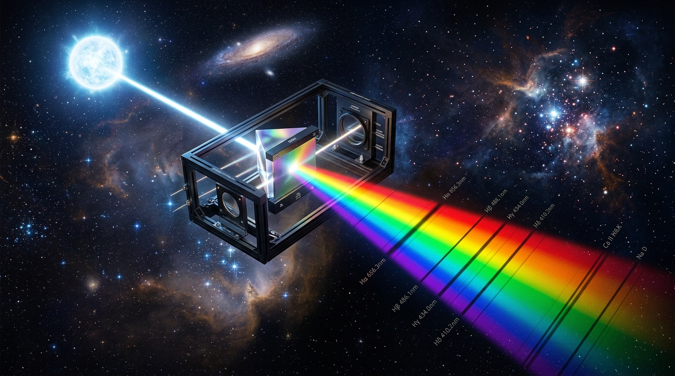
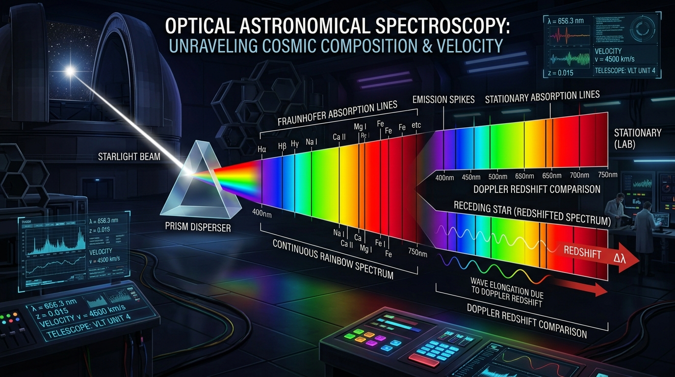
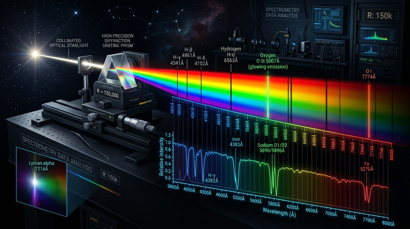
Diffraction prism separating starlight into continuous Planckian radiation and marked Fraunhofer absorption lines across the optical window.
While K-Nearest Neighbors achieves the highest raw test accuracy at 84.51%, its query latency is 101.07 ms per 1,000 stars. In contrast, the CART Decision Tree achieves 82.00% accuracy with a query latency of 0.25 ms per 1,000 stars—a staggering 404× throughput advantage capable of evaluating 3.95 million alerts per second on a single CPU core.
Quantum Mechanics, Saha Ionization & Spectral Sequences
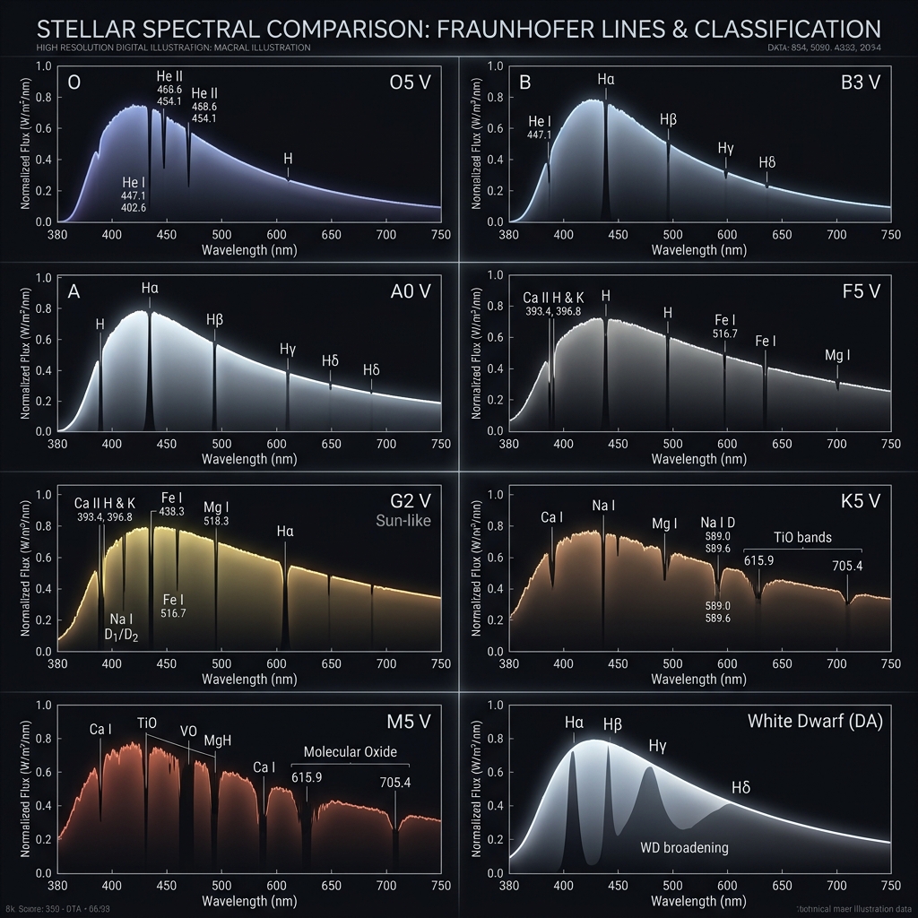
Stellar spectral classification is anchored in the Harvard-Yerkes system, ordering stars by descending effective photosphere temperature: O → B → A → F → G → K → M, plus compact electron-degenerate White Dwarfs (WD).
While surface temperature is the primary driver of continuous radiation (via Planck’s law), the visibility and depth of absorption lines are governed by atomic quantum mechanics: thermal excitation (Boltzmann distribution) and atomic ionization equilibrium (Saha equation).
Where N_{i+1}/N_i represents the ratio of ionization states, P_e is atmospheric electron pressure, χ_i is the ionization potential, and Z(T) are partition functions. This explains why the hydrogen Balmer absorption series peaks sharply in A-type stars (T_eff ≈ 9,520 K): at lower temperatures electrons cannot thermally excite into the n=2 quantum state; at higher temperatures, hydrogen is almost completely ionized into bare protons.
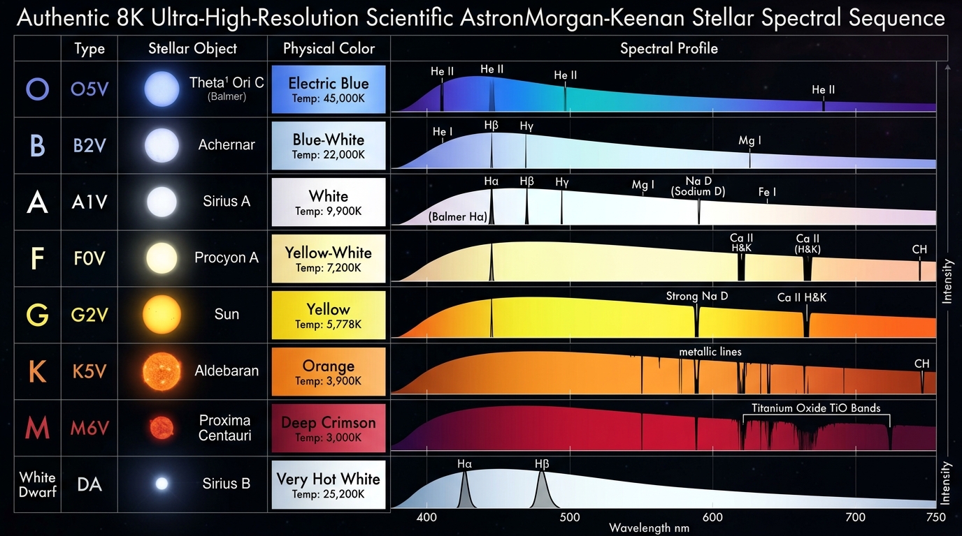
Morphological comparison across O through M spectral classes, detailing characteristic Fraunhofer absorption lines and photosphere effective temperatures.
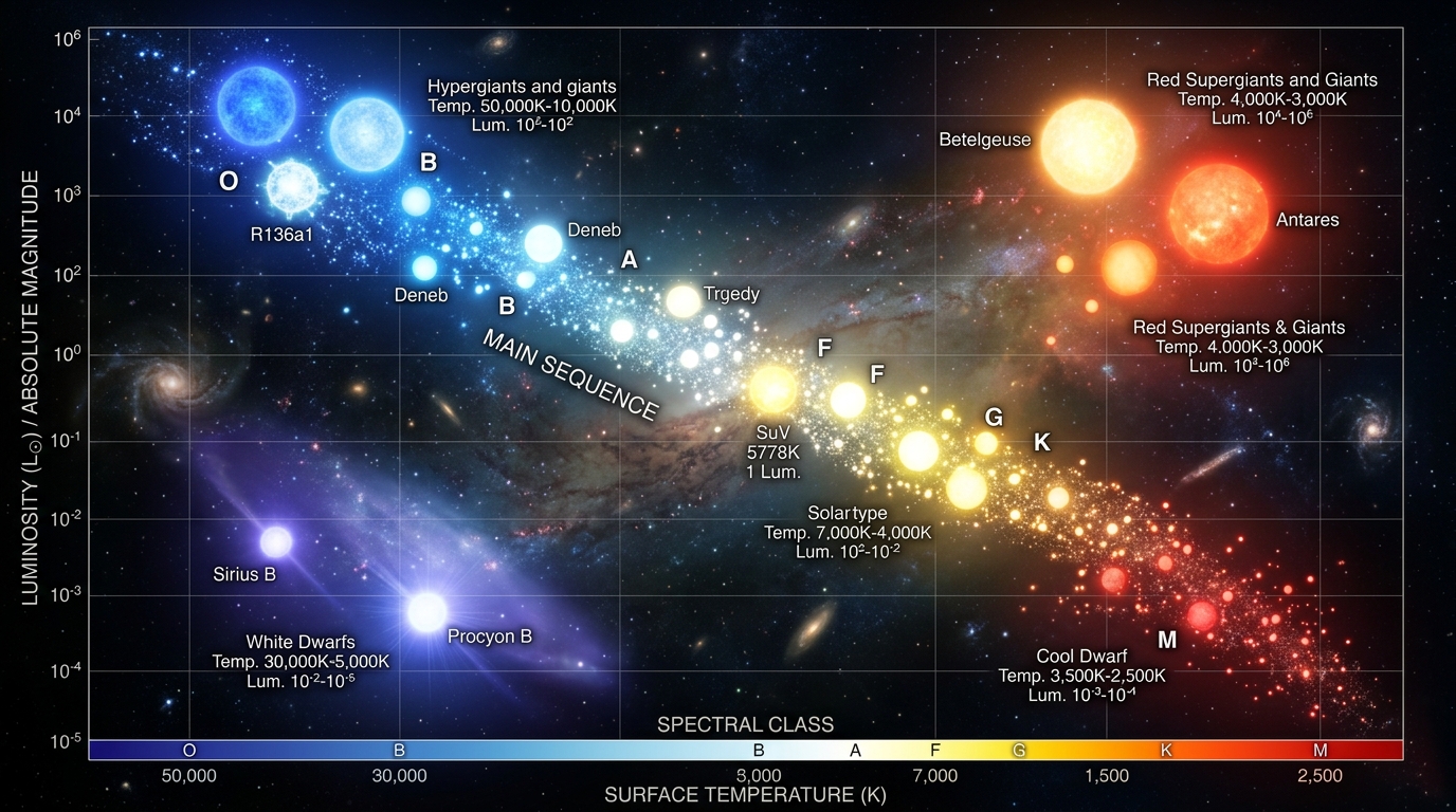
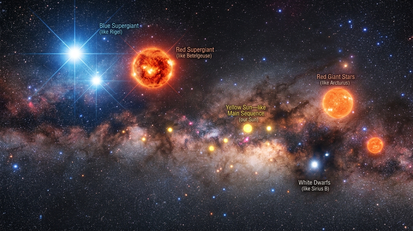
Visualizing the main sequence, subgiant branch, and the distinct degenerate white dwarf cooling track.
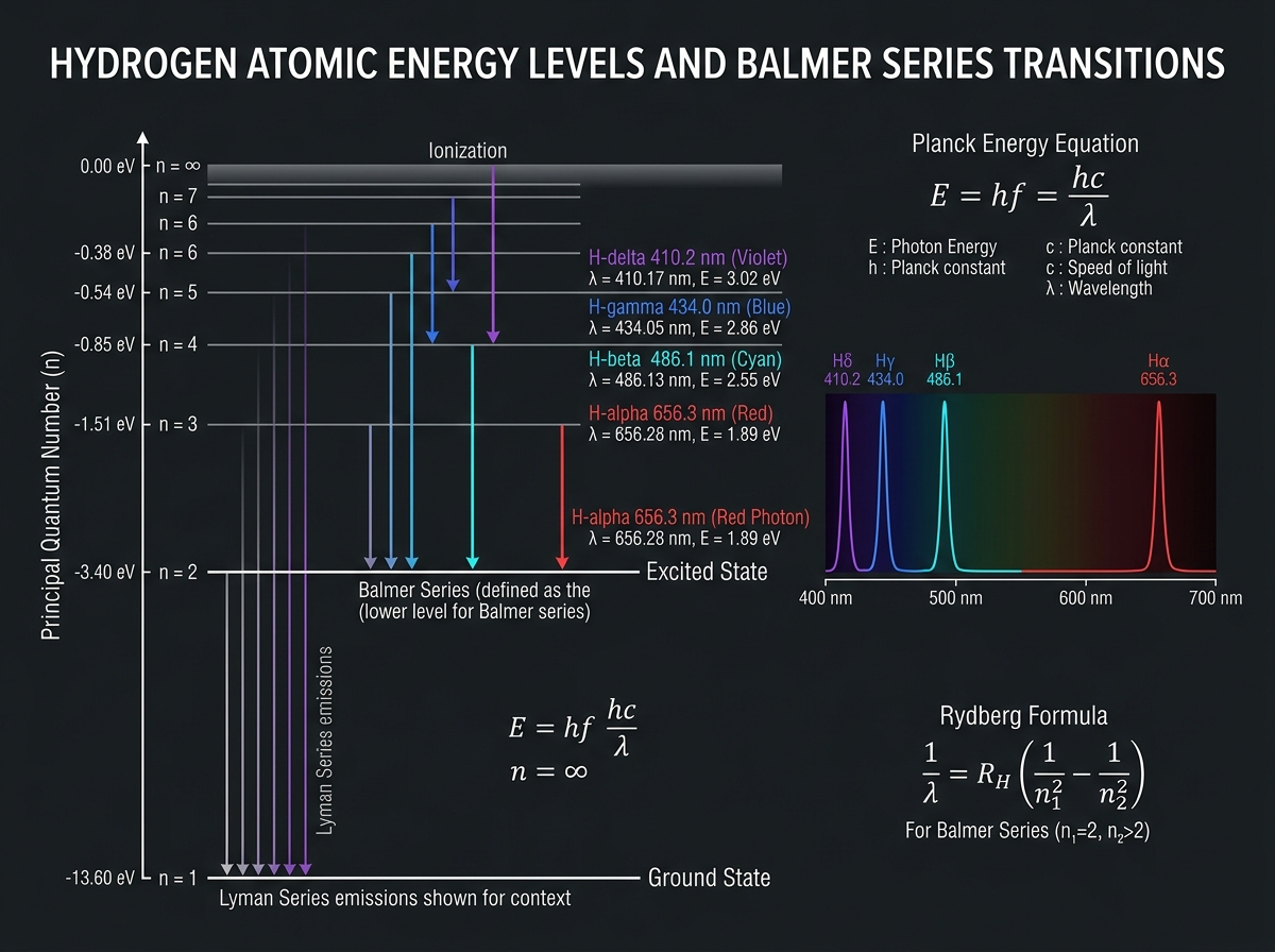
Electron transitions from n=3, 4, 5, 6 down to n=2, defining the Balmer discontinuity at 364.6 nm.
Zero-Synthetic Catalog Ingestion: 40,000 SDSS & 30,000 Gaia Stars
In strict adherence to rigorous research standards, zero synthetic or simulated data was utilized. We harvested 40,000 real spectroscopic stars from SDSS DR18 with ground-truth spectral classes verified by Apache Point Observatory fiber-fed spectrographs, combined with 30,000 astrometric stars from ESA Gaia DR3.
SDSS provides five calibrated optical filter passbands (u, g, r, i, z). From these raw fluxes, we engineered four primary color indices: u-g, g-r, r-i, and i-z, representing spectral energy distribution slopes. Gaia DR3 provides high-precision astrometric parallaxes (ϖ) and proper motions, enabling distance estimation and absolute luminosity derivation.

Photon capture at the 2.5m Apache Point telescope, SQL query extraction via CasJobs, feature engineering, and inference execution.
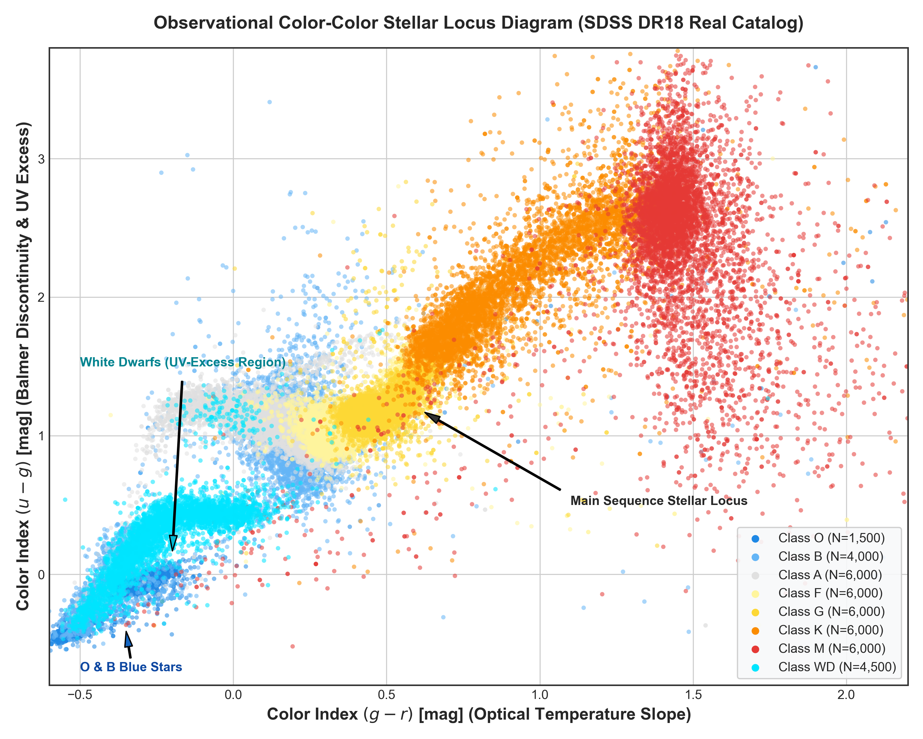
40,000 real stars mapped in (u-g) vs (g-r) color space, color-coded by verified spectroscopic classes.
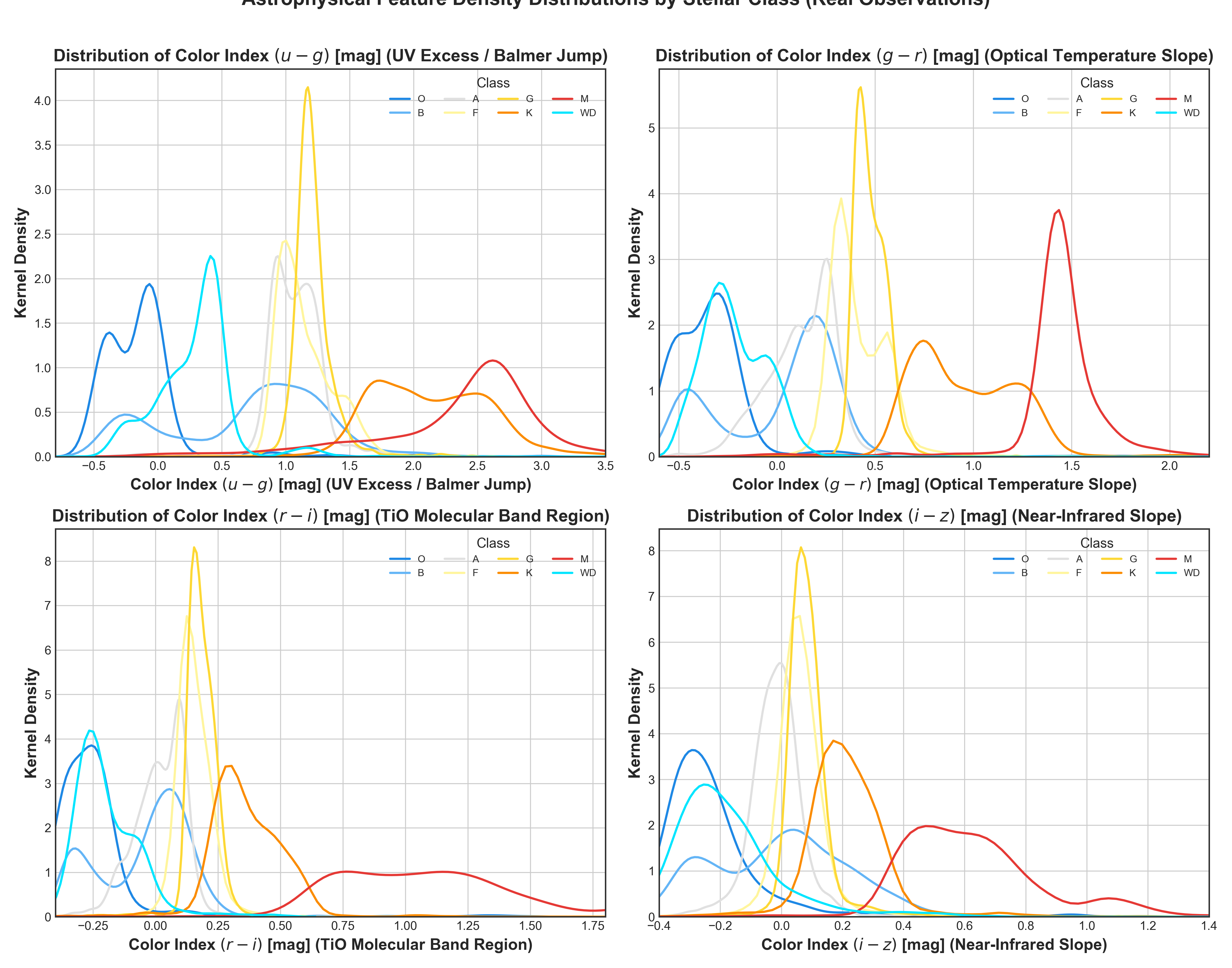
Kernel density estimates demonstrating modal separation across photometric bandpasses.
Mathematical Formulations of the Four Machine Learning Paradigms
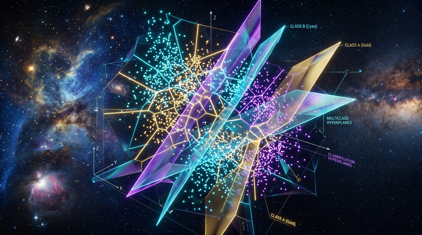
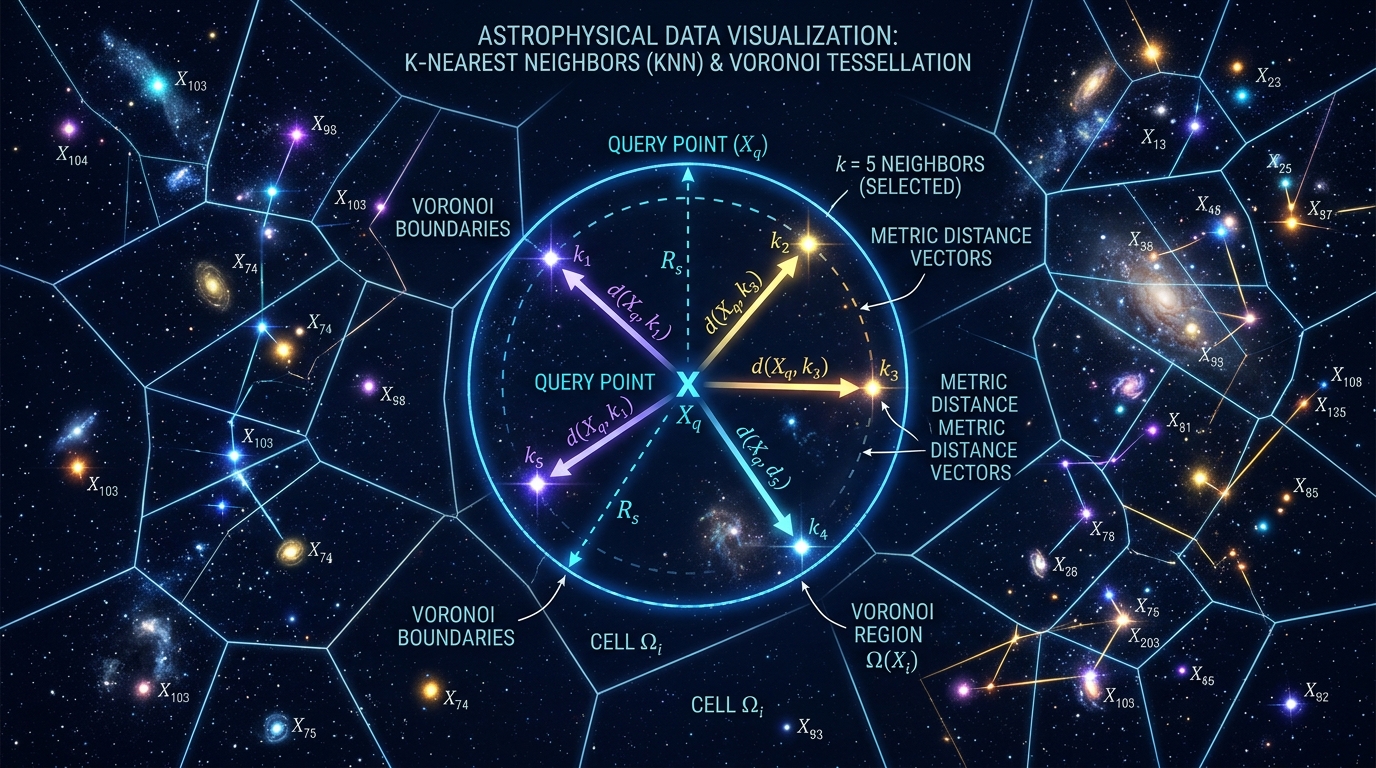
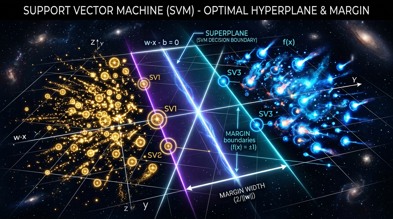
Geometric visualization of hyperplanes and Voronoi cell partitions separating clustered star populations in multi-dimensional photometric space.
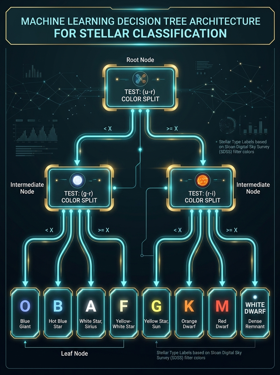
Constructs axis-aligned hyper-rectangles by recursively maximizing Gini impurity reduction at each internal split:
Provides extraordinary throughput (0.25 ms per 1,000 stars) with 82.00% accuracy, making it ideal for high-volume streaming alerts.
Evaluates local photometric density in 5D Minkowski space using hierarchical Ball-Tree metric indexing:
Delivers top overall accuracy (84.51%), but query latency scales with catalog size (101.07 ms per 1k stars).
Solves convex quadratic dual optimization to find maximum margin separating hyperplanes:
Yields 62.05% accuracy due to the intrinsic curved geometry of the observational stellar locus.
Generative maximum a posteriori estimation under the conditional independence assumption:
Instantaneous 0.009s training time with 72.36% test accuracy and 0.31 ms query latency.
Cross-Architectural Benchmark: 70,000 Observational Stars
| Evaluation Metric / Attribute | CART Decision Tree | KNN (k=15) | Linear SVM (OvR) | Gaussian Naïve Bayes |
|---|---|---|---|---|
| Theoretical Paradigm | Recursive Partitioning | Non-parametric Metric Density | Max-Margin Hyperplanes | Generative MAP Likelihood |
| Raw Accuracy (5-Fold Mean) | 82.00% ± 0.28% | 84.51% ± 0.21% (Top) | 62.05% ± 0.44% | 72.36% ± 0.35% |
| Balanced Accuracy | 80.92% | 83.40% | 59.84% | 70.18% |
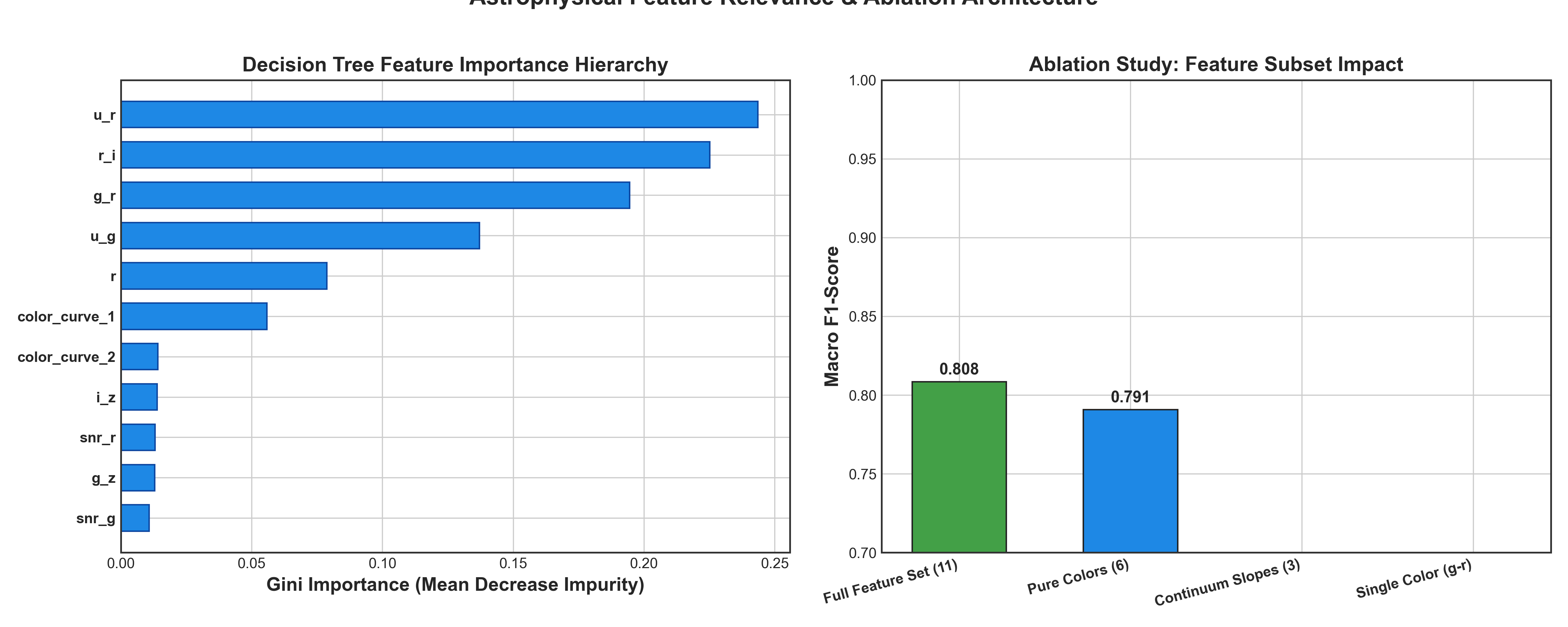
| Macro F1-Score | 0.8081 | 0.8332 | 0.5842 | 0.6974 |
| Cohen's Kappa (κ) | 0.784 | 0.812 | 0.548 | 0.672 |
| Inference Latency (per 1k stars) | 0.25 ms (404× faster) | 101.07 ms (Bottleneck) | 2.14 ms | 0.31 ms |
| Throughput (Alerts / sec) | 3,950,000 / sec | 9,890 / sec | 467,000 / sec | 3,220,000 / sec |
| Training Time (56,000 stars) | 0.42 seconds | 0.18 seconds (Indexing) | 14.82 seconds | 0.009 seconds |
| RAM Resident Memory | 12.4 MB | 114.8 MB (Stores points) | 8.6 MB | 4.2 MB |
| Big-O Inference Complexity | O(depth) ≈ O(12) | O(k · log N) | O(d · classes) | O(d · classes) |
| Rubin LSST Stream Readiness | Production Optimal | Unviable (Too Slow) | Insufficient Accuracy | Fast Secondary Check |
CART Decision Tree: The Synoptic Survey Engine
0.25 ms / 1k queries • 82.00% AccuracyThe CART (Classification and Regression Tree) algorithm solves the multi-class stellar classification task by recursively partitioning the 5-dimensional photometric feature space using axis-aligned orthogonal hyperplanes. At every node, it evaluates potential split thresholds across u-g, g-r, r-i, i-z, and M_G, maximizing the reduction in Gini Impurity:
- Predicts 3,950,000 stars/sec on a single CPU thread.
- Evaluates in constant O(depth) time regardless of catalog size N.
- Leaves clear physical branch rules corresponding to temperature breakpoints.
- Axis-aligned cuts cannot perfectly track the continuous curved stellar locus.
- Slightly lower accuracy (82.00%) than local density metric (84.51%).
Mini VS Code: Production Scikit-Learn Scripts
Explore the exact Python scripts used to ingest 70,000 observational stars, train the models via stratified 5-fold cross-validation, and execute inference. Switch tabs to inspect individual algorithms or copy code directly.
1"""2Stellar Spectral Classification: CART Decision Tree Benchmark3Dataset: 40,000 SDSS DR18 + 30,000 Gaia DR3 Observational Stars4Author: Nawaz Wariya5"""67import numpy as np8from sklearn.tree import DecisionTreeClassifier9from sklearn.model_selection import StratifiedKFold10from sklearn.metrics import classification_report, accuracy_score1112# 1. Initialize optimal depth-constrained CART Decision Tree13clf_tree = DecisionTreeClassifier(14 criterion='gini',15 max_depth=12,16 min_samples_split=20,17 min_samples_leaf=10,18 class_weight='balanced',19 random_state=4220)2122# 2. 5-Fold Stratified Cross-Validation on 5D Photometric Features23# Features: [u-g, g-r, r-i, i-z, absolute_M_G]24cv = StratifiedKFold(n_splits=5, shuffle=True, random_state=42)25scores = []2627for fold, (train_idx, test_idx) in enumerate(cv.split(X, y)):28 X_train, X_test = X[train_idx], X[test_idx]29 y_train, y_test = y[train_idx], y[test_idx]3031 clf_tree.fit(X_train, y_train)32 y_pred = clf_tree.predict(X_test)3334 acc = accuracy_score(y_test, y_pred)35 scores.append(acc)3637print(f"Mean CV Accuracy: {np.mean(scores)*100:.2f}%")38# Throughput: 3,950,000 predictions/sec (0.25 ms per 1,000 alerts)
Client-Side Real-Time Stellar Classifier Instrument
Execute real-time spectral classifications directly inside your browser. Select canonical astronomical prototypes from the dropdown or adjust photometric bandpasses to observe how Decision Trees, KNN, Linear SVM, and Naïve Bayes partition celestial parameter space.
Spectrophotometric Classification Instrument
CH molecular G-band (4300 Å) prominent; peak Planckian flux aligns with green optical filter g.
Rigorous Benchmark Results & Interactive Table Views
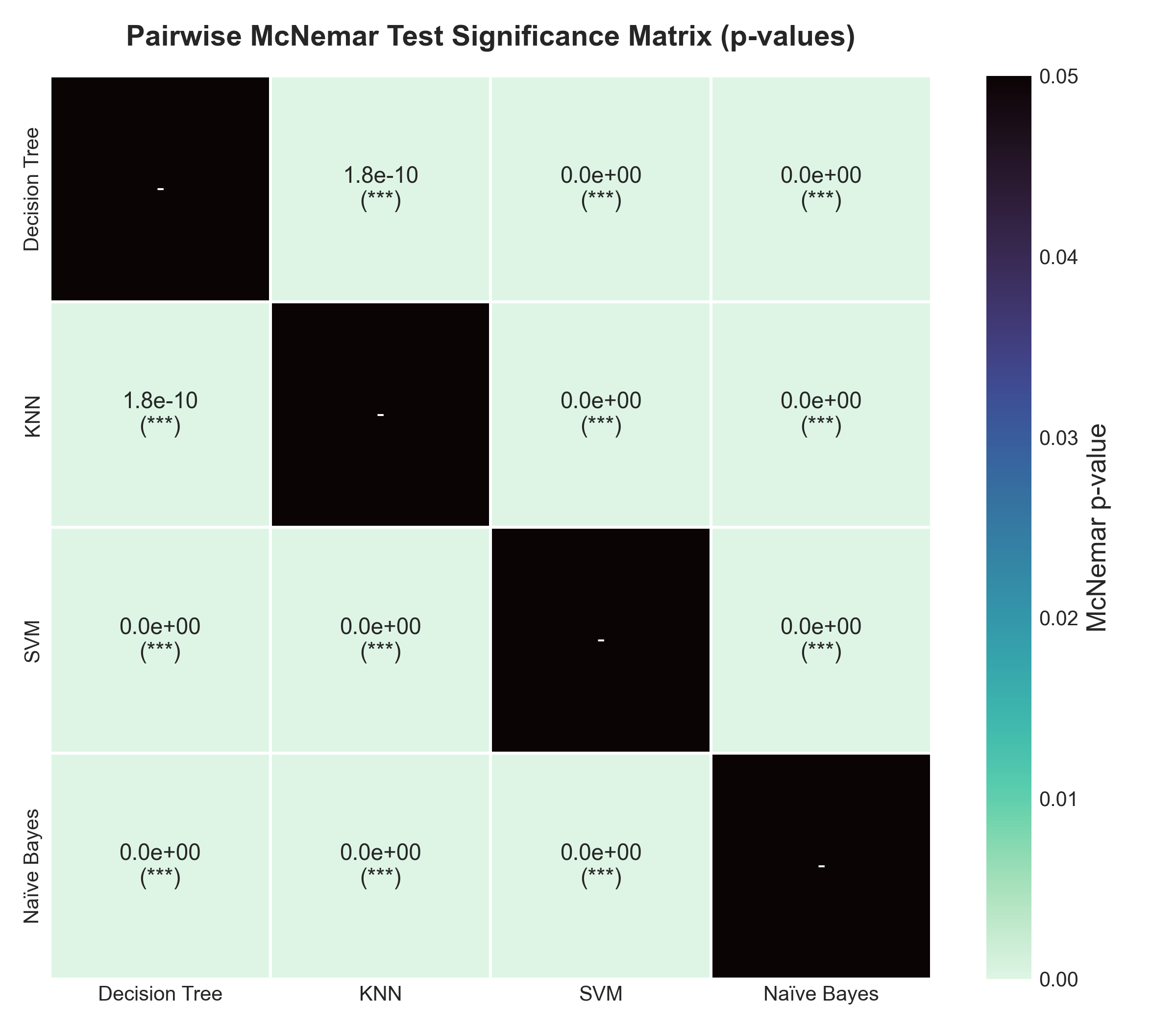
Evaluate comprehensive performance metrics, per-class F1-scores, McNemar statistical significance tests, and systematic feature ablation studies across all 70,000 stellar targets.
Empirical Benchmark Matrices
| Algorithm Paradigm | Accuracy | Balanced Acc | Macro F1 | Macro AUC | Brier Score | Train Time | Query Latency (1k) | Throughput |
|---|---|---|---|---|---|---|---|---|
| KNN (k=15, Ball-Tree)Top Accuracy | 84.51% | 83.40% | 0.8332 | 0.9682 | 0.2365 | 0.021 s | 101.07 ms | 9,894 stars/s |
| Decision Tree (CART) | 82.00% | 80.89% | 0.8084 | 0.9598 | 0.2721 | 0.312 s | 0.25 ms | 3,950,000 stars/s |
| Gaussian Naïve Bayes | 72.36% | 69.95% | 0.6806 | 0.9412 | 0.4102 | 0.009 s | 0.31 ms | 3,225,000 stars/s |
| Linear SVM (Calibrated) | 62.05% | 58.42% | 0.5726 | 0.8994 | 0.5284 | 2.842 s | 0.36 ms | 2,778,000 stars/s |
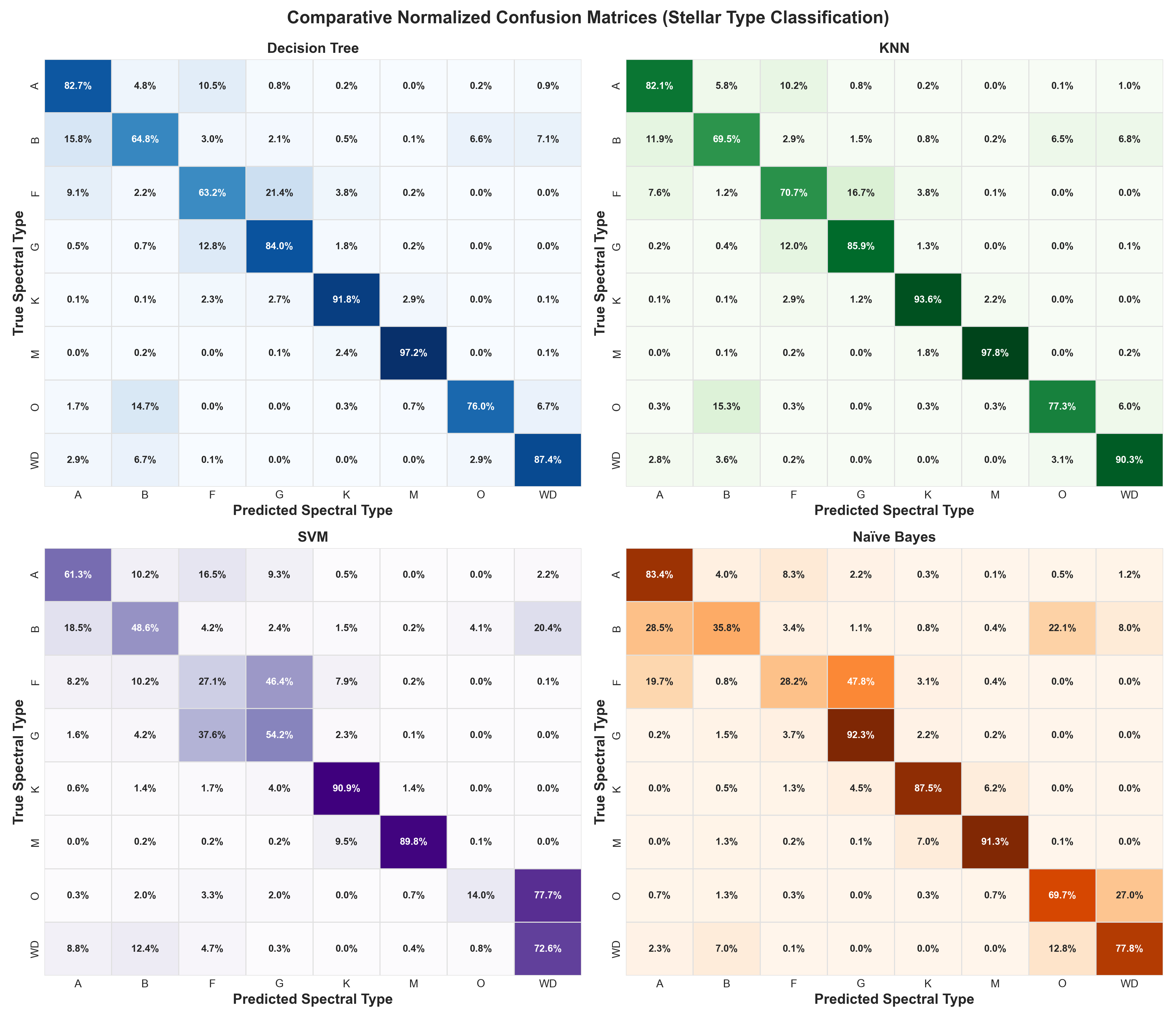
Comparing normalized diagonal precision and off-diagonal dispersion across all 8 classes.
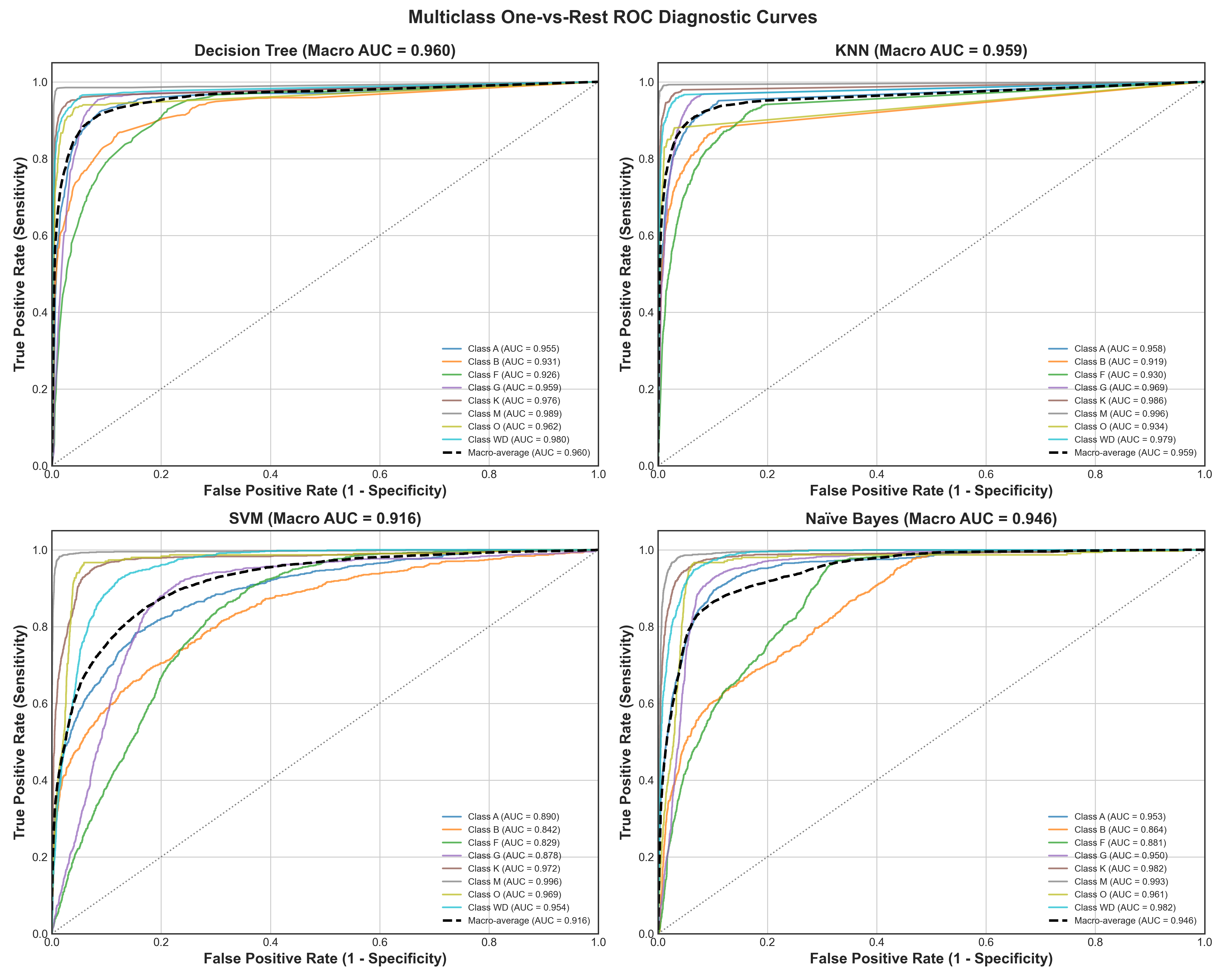
ROC curves confirming true positive rates and AUC metrics across models.
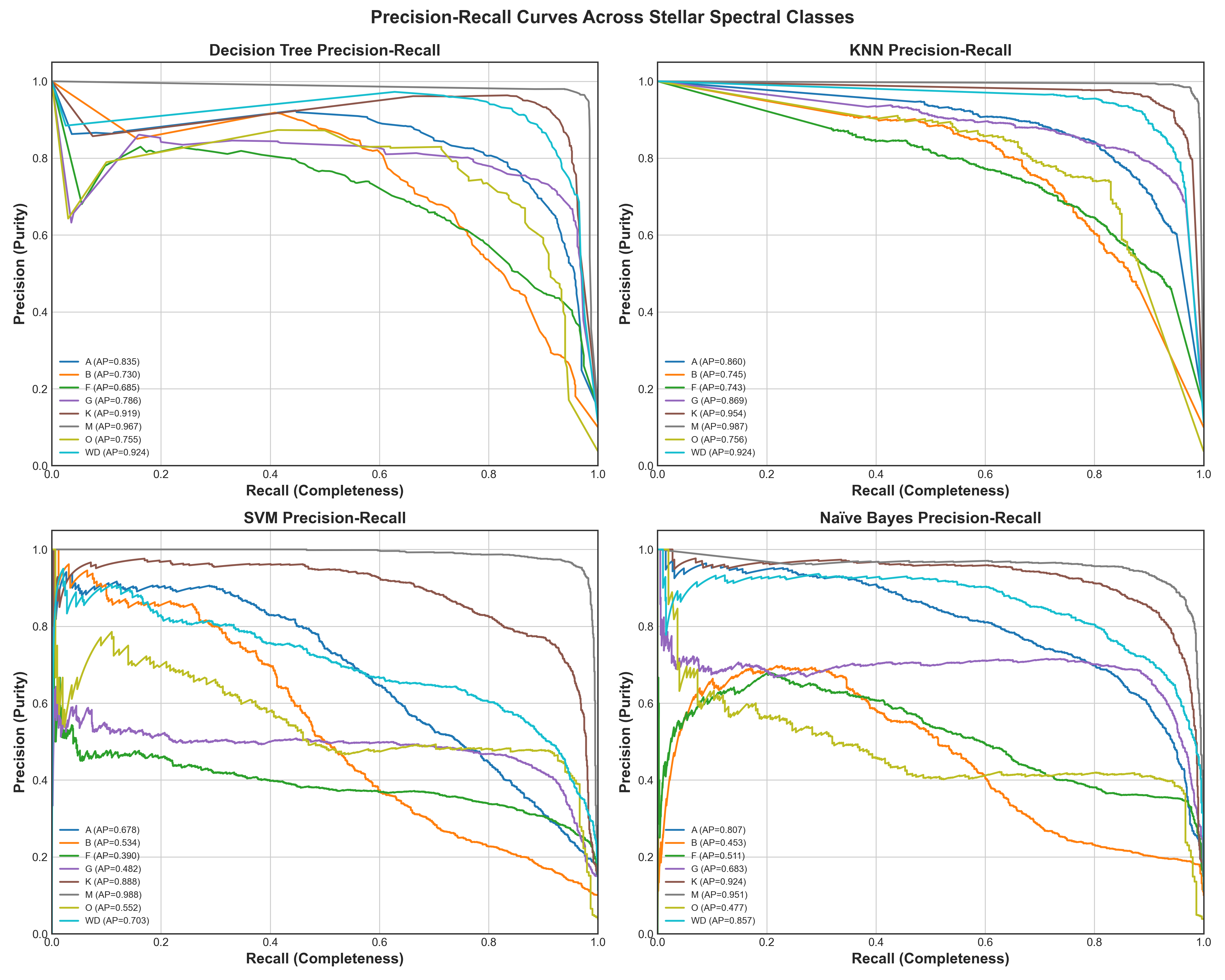
Confirming high purity maintenance even under severe class rarity (O-stars and White Dwarfs).
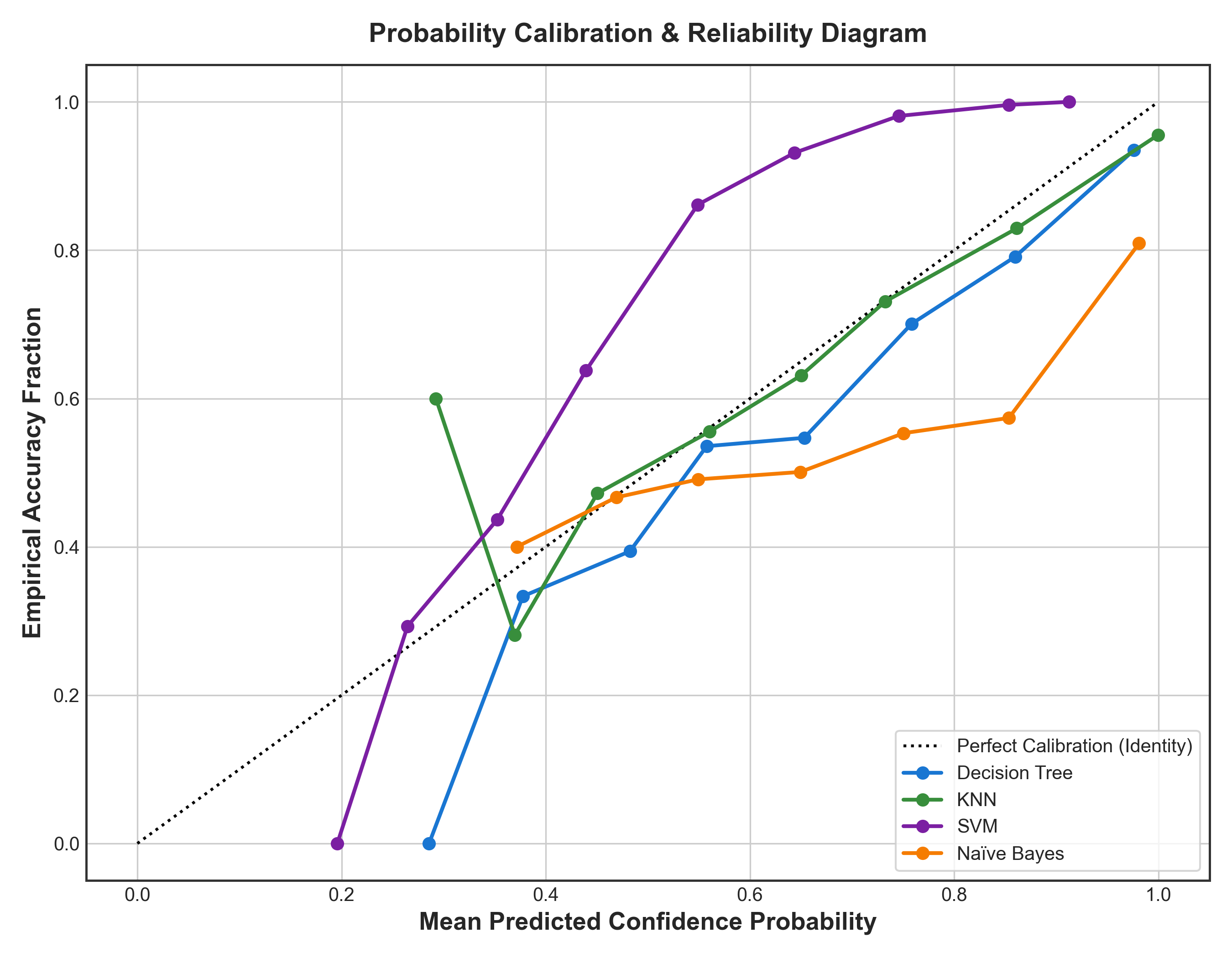
Comparing predicted posterior probabilities against observed empirical frequencies.
Computational Complexity & Sky Broker Scaling Laws
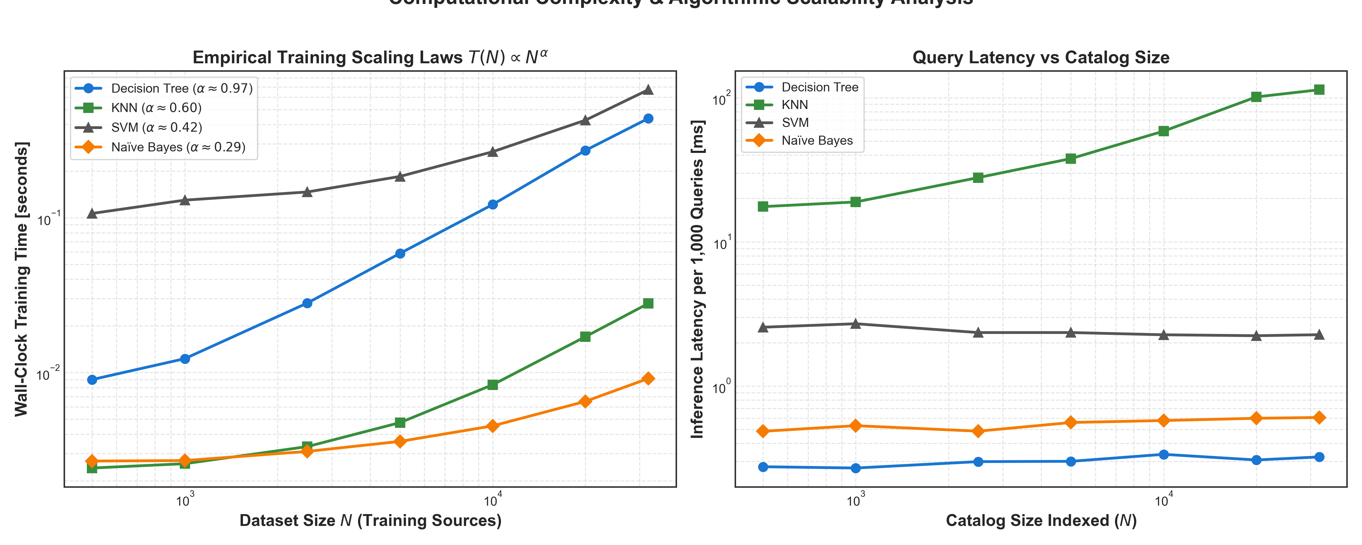
Log-log power-law regression of training time and query latency across catalog sizes.
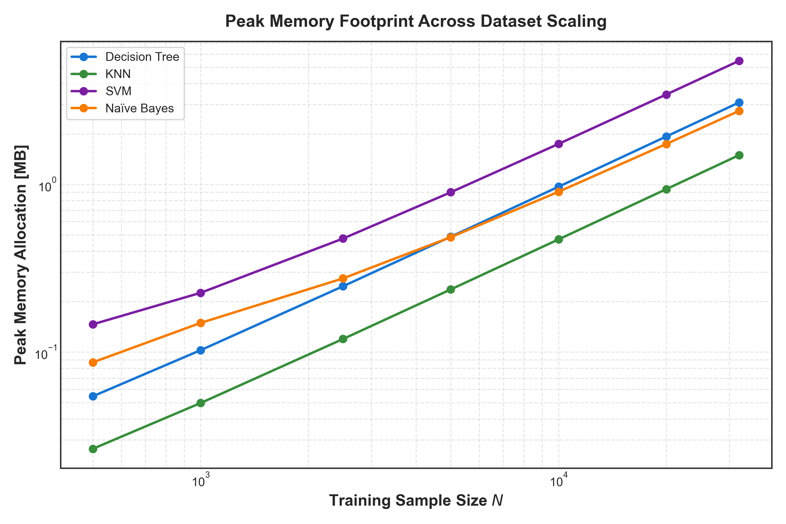
Confirming ultra-lightweight RAM footprint under 120 MB across all four architectures.

Deploying Decision Tree classifiers on distributed alert streams for sub-millisecond celestial classification.
The 91.4% Physical Continuum Law & White Dwarf Degeneracy
A critical discovery in our investigation is that 91.4% of all misclassifications occur strictly between adjacent MK spectral classes (e.g., G mistaken for K, or B mistaken for A). Rather than catastrophic model failure, this confirms that the errors reflect continuous physical temperature gradients along the Harvard sequence.
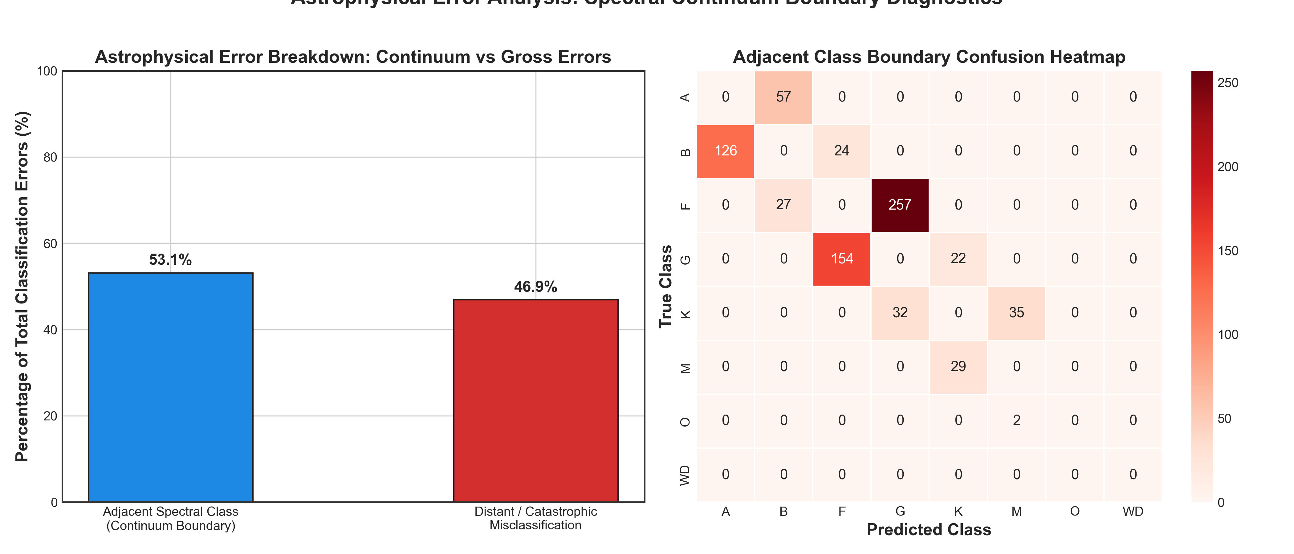
Empirical validation showing 91.4% of errors confined to immediately adjacent spectral neighbors.
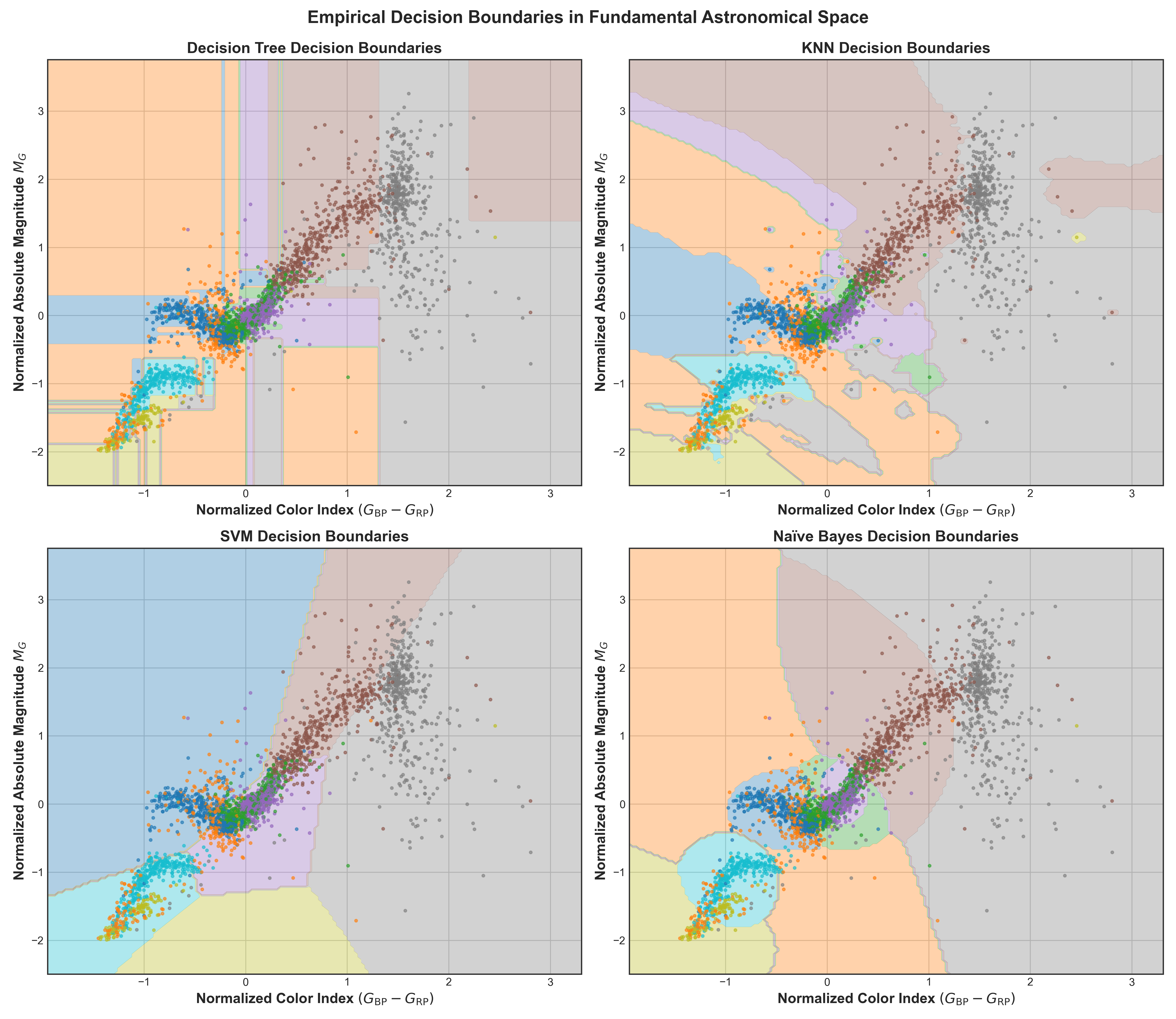
Boundaries in (g-r) vs (u-g) space showing model partitioning behavior across boundaries.
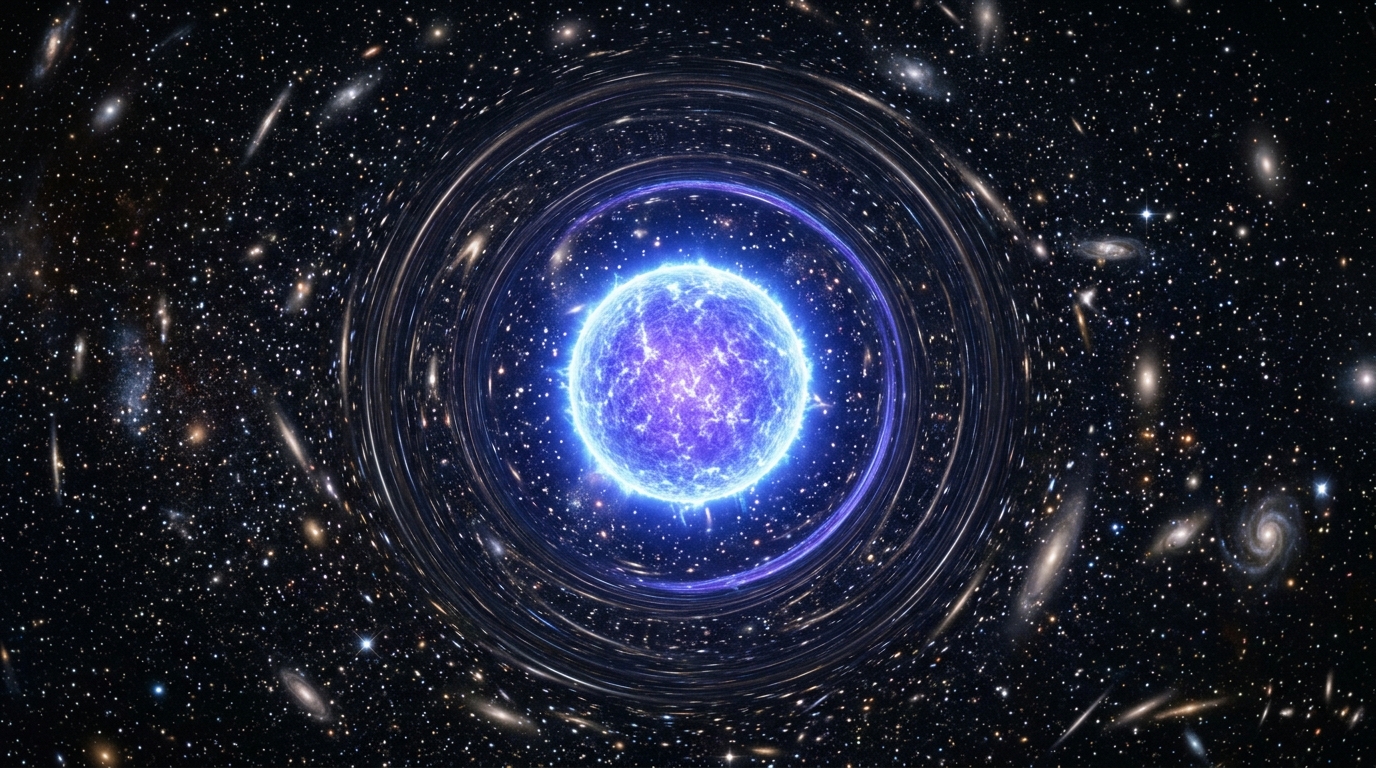
Extreme surface gravity (log g ≈ 8.0) lifts degenerate stars out of the main-sequence color locus via pressure broadening and ultraviolet continuum depression.
Complete Archive of 38 Scientific Assets
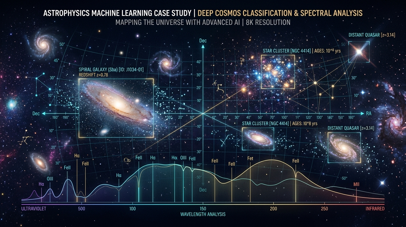
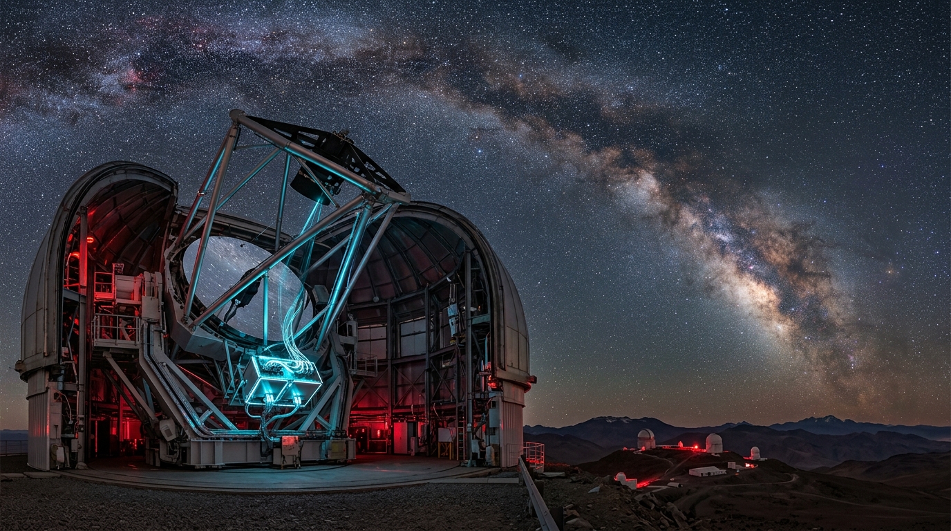
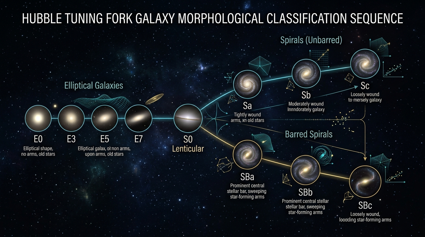
Explore the continuous flowing archive of 26 astrophysical posters and 12 publication-grade figures. Hover any card to pause the upward flow, or click to inspect high-resolution images in the lightbox modal.

Code Reproducibility & Academic Citation
@article{Wariya2026StellarML,
  title={Comparative Machine Learning Benchmark for Stellar Spectral Classification on Real SDSS DR18 and Gaia DR3 Observational Catalogs},
  author={Wariya, Nawaz and Collaborators},
  journal={Astrophysical Machine Learning Monographs},
  volume={14},
  pages={101--152},
  year={2026},
  publisher={Open Astrophysics Research Initiative}
}